Visualizing Cable Outages using Power Query

I’ve long been a fan of PowerQuery (PQ), even more so since Microsoft finally made it available on Mac. If you’re unfamiliar, here’s a worked example of how to use it for a, sadly, every day problem.

Since moving house this summer we’ve gone from a rock solid fiber Internet connection to a less than glorious Xfinity cable connection that suffers an outage or two every day (as my team can attest to with frozen Teams calls). It’s infuriating.

Getting customer service from any cable company is always a challenge (‘have you rebooted your router?’) so I resolved to collect some outage data that will perhaps nudge Xfinity to take me seriously.

The first thing to do is collect good quality data. I installed the netcheck package on my hardwired Raspberry PI  and started to collect data. The software logs outages like this: 

-----------------------------------------------------------------------------
LINK DOWN:                                       Wed 20 Sep 2023 10:29:17 CDT
LINK RECONNECTED:                                Wed 20 Sep 2023 10:30:51 CDT
TOTAL DOWNTIME:                                  1 minutes and 34 seconds.
RECONNECTED LINK SPEED:                         
-----------------------------------------------------------------------------
                                                 Ping: 22.03 ms
                                                 Download: 26.02 Mbit/s
                                                 Upload: 39.22 Mbit/s
-----------------------------------------------------------------------------

The key data we need is those LINK DOWN and RECONNECTED lines. Those are easily extracted with a Grep statement:

grep -P "LINK (D|R)" connection.log > temp.log

That gives us a log file like this:

LINK DOWN:                                       Tue 19 Sep 2023 07:39:40 CDT
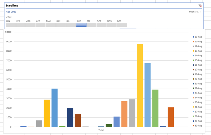
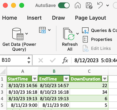
LINK RECONNECTED:                                Tue 19 Sep 2023 07:42:26 CDT

My goal is to get to a three column file, outage start, outage end, duration (in seconds), so I can chart the data, perhaps using a Pivot Chart:

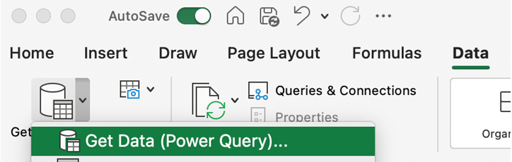
To manipulate the file using PowerQuery, first open Excel and select the Get Data (Power Query) option under the Data Tab (my screenshots are Mac but they are almost identical for PC).

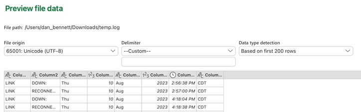
Select the Text/CSV option, choose the file and you’re presented with a preview of the data:

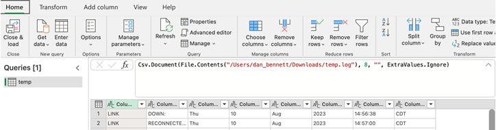
Click the transform button to launch the PowerQuery Editor. What I love about this environment is that if you prefer to edit your data visually, you can, yet the editing steps are stored as code you can directly edit if you wish.

A bit like Excel, each line of code (in this case, loading a document) is shown in the function bar with the resulting data shown below:

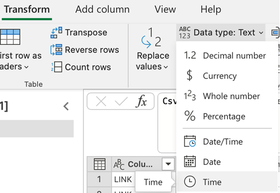
Notice all the columns are imported as text (the ‘ABC’ icon in the column header. The first thing to do convert the time to a timestamp. Click that column, click Transform and change the type to time:

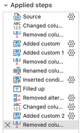
Some of the columns we don’t need: the timezone, day and ‘LINK’ columns. Click each column header and select remove column. As you transform the data, you’ll see each step being recorded on the right hand side:

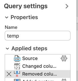
This is one of the things I love about PQ. Click on each step and you can see the exact changes you’ve made to your data.

The next thing to do is to recombine those three date columns into a new column with the date type. Click ‘Custom Column’ on the ‘Add Column’ tab. A quick search of the PQ website shows me the function to convert a string to a date:

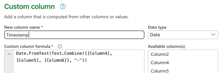
Next, I combine the date and time columns with a new custom column called StartTime. The formula is as simple as  [Timestamp] & [Column7]

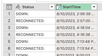
I can now remove the columns I don’t need. Unlike Excel, PQ actually copies the data when you create a new column, so removing superfluous columns won’t ‘break’ your formula. It’s always good practice to remove unneeded columns to reduce storage and keep things tidy, leaving me with two columns.

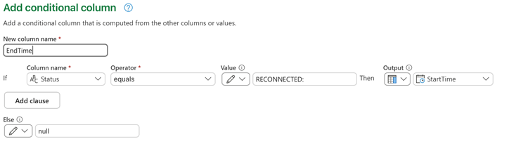
To chart this data, I need to combine each pair of rows so I have a start and end time. There’s multiple ways of doing this. An easy way is to use Fill Up to copy data from a subsequent row. To do that, we need a new column that will become the end time. I use a conditional column here to only copy the end time if it truly is:

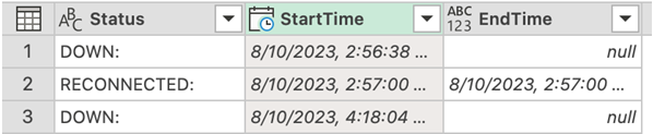
This results in a half filled End Time column:

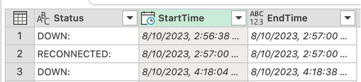
Next, I use a ‘Fill Up’ (under the Transform tab, Fill button) command to replace the ’null’ values with the value from the row below:

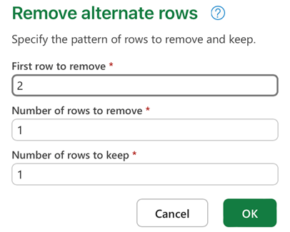
Only two steps remain. We need to remove the ‘RECONNECTED’ rows as we don’t need them any more and then calculate the duration of the outage.

There are multiple ways to achieve the first goal, an easy way is ‘Remove Alternate Rows’ under the ‘Remove Rows’ button

Finally we add a custom column for duration with the following formula to count seconds: Duration.TotalSeconds(Duration.From([EndTime]-[StartTime]))

After removing the Status column we end up with three columns. Click ‘Close and Load’ to insert them into Excel:

One thing is missing.. we don’t have rows for days when there were no outages. That’s a post for another day… and with the number of outages there’s not many needed anyway!

Here’s all the steps. While it might seem a lot, each is a very simple transformation that we can easily understand and change or delete if we make a mistake:

Hopefully this has inspired you to give PQ a try. yourself. Let me know how you get on.